The origin of the boosting method for designing learnign machines is traced back to the work of Valiant and Kearns, who posed the question of whether a weak learning algorithm, meaning one that does slightly better than random guessing, can be boosted into a strong one with a good performance index.
- At the heart of such techniques lies the base leaner, which is a week one.
Boosting consists of an iterative scheme, where
- at each step the base learn is optimally computed using a different training set;
Boosting consists of an iterative scheme, where at each step the base learner is optimally computed using a different training set;
- the set at the current iteration is generated either:
- according to an iteratively obtained data distribution or,
- usually, via a weighting of the training samples, each time using a different set of weights.
The final learner is obtained via a weighted average of all the hierarchically designed base learners.
It turns out that, given a sufficient number of iterations, one can significantly imporve the (poor) performance of a weak learner. (?)
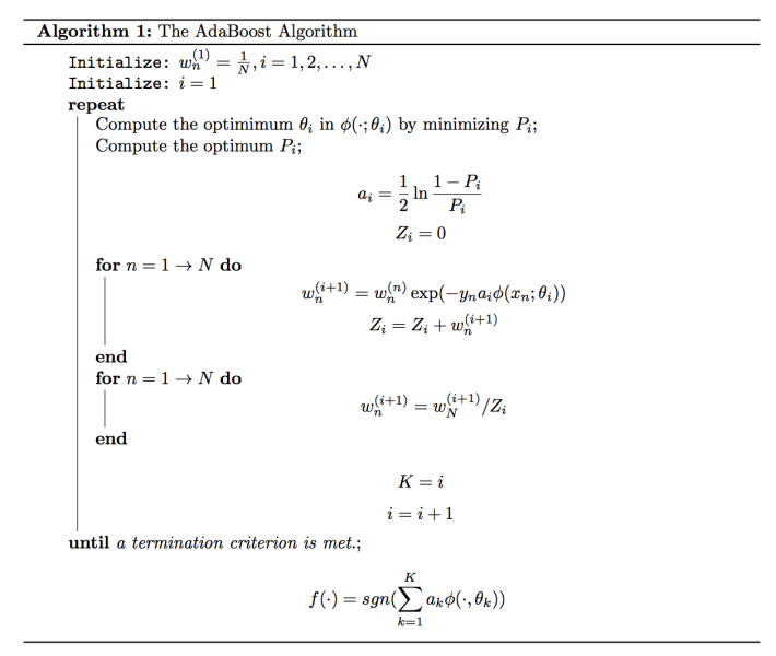
The AdaBoost Algorithm
Our goal is to design a binay classifier:
where
where 

- The base classifier is selected to be a binary one.
- The set of unknown paramters is obtained in a step wise approach and in a greedy way; that is:
- At each iteration step,
, we only optimize with respect to a single pair,
, by keeping the parameters,
., obtained from the previous steps, fixed.
- At each iteration step,
Note that ideally, one should optimize with respect to all the unknown parameters, 
Assume that we are currently at the

Then we can write the following recursion:

starting from an intial condition. According to the greedy retionale, 

For optimization, a loss function has to be adopted. No doube different options are avialable, giving different names to the derived algorithm. A popular loss function used for classification is the exponential loss, defined as

and it gives rise to the Adaptive Boosting algorithm. The former can be considered a (differentiable) upper bound of the (nondifferentiable) 0-1 loss function.
- Note that the exponential loss weights misclassified (
) points more heavily compared to the correctly identified ones (
).
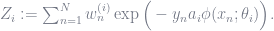
Employing the exponential loss function, the set 

This optimization is also performed in two steps. First , 


where

Observe that 


The optimization depends on the specific form of the base classifier. However, due to the exponential form of the loss, and the fact that the baseclassifier is a binary one, so that 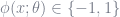

where
![P_i := \sum_{n=1}^N w_n^{(i)} \chi_{(-\infty, 0]}\bigg(y_n \phi\big(x_n;\theta\big)\bigg),](https://s0.wp.com/latex.php?latex=P_i+%3A%3D+%5Csum_%7Bn%3D1%7D%5EN+w_n%5E%7B%28i%29%7D+%5Cchi_%7B%28-%5Cinfty%2C+0%5D%7D%5Cbigg%28y_n+%5Cphi%5Cbig%28x_n%3B%5Ctheta%5Cbig%29%5Cbigg%29%2C+&bg=ffffff&fg=6e7381&s=0&c=20201002)
and ![\chi_{(-\infty, 0]}(\cdot)](https://s0.wp.com/latex.php?latex=%5Cchi_%7B%28-%5Cinfty%2C+0%5D%7D%28%5Ccdot%29+&bg=ffffff&fg=6e7381&s=0&c=20201002)


- To guarantee that
interval, the weights are normalized to unity by dividing by the respective sum; note that this does not affect the optimization process.
In other words, 
Having computed the optimal 

and


Taking the derivative with respect to

Once 
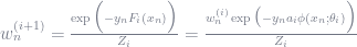
where 
Looking at the way the weights are formed, one can grasp one of the major secrets underlying the AdaBoost algorithm:
- The weight associated with a training sample,
, is increased (decreased) with respect to its value at the previous iteration, depending on whether the pattern has failed (succeeded) in being classified correctly.
- Moreover, the percentatge of the dececrease (increase) depends on the value of
, which controls the relative importance in the buildup of the final classifier.
- Hard samples, which keep failing over successive iterations, gain importance in their participation in the weighted empirical error value.
- For the case of the AdaBoost, it can be shown that the training error tends to zero exponentially fast. (?)
Algorithm 7.1 (The AdaBoost algorithm)

The Log-Loss Function
In AdaBoost, the exponential loss function was employed. From a theoretical poiont of view, this can be justified by teh following argument:
- Consider the mean value with respect to the binary label,
, of the exponential loss function:
![E\big[\exp (-y F(x))\big] = P(y = 1) \exp(-F(x)) + P(y = -1) \exp(F(x))](https://s0.wp.com/latex.php?latex=E%5Cbig%5B%5Cexp+%28-y+F%28x%29%29%5Cbig%5D+%3D+P%28y+%3D+1%29+%5Cexp%28-F%28x%29%29+%2B+P%28y+%3D+-1%29+%5Cexp%28F%28x%29%29+&bg=ffffff&fg=6e7381&s=0&c=20201002)
Taking the derivative with resepct to 
![F_*(x) = \arg\min_f \mathbb{E}[\exp(-yf)] = \frac{1}{2}\ln \frac{P(y = 1 | x)}{P(y = -1 | x)}](https://s0.wp.com/latex.php?latex=F_%2A%28x%29+%3D+%5Carg%5Cmin_f+%5Cmathbb%7BE%7D%5B%5Cexp%28-yf%29%5D+%3D+%5Cfrac%7B1%7D%7B2%7D%5Cln+%5Cfrac%7BP%28y+%3D+1+%7C+x%29%7D%7BP%28y+%3D+-1+%7C+x%29%7D+&bg=ffffff&fg=6e7381&s=0&c=20201002)
The logarithm of the ratio on the right-hand side is known as the log-odds ratio. Hence, if one views the minimizing function in (7.88) as the empirical approximation of the man value in (7.89), it fully justifies considering the sign of the fucntion in (7.73) as the classification rule.
A major problem associated with the exponential loss function, as is readily seen in Figure (7.14), is that it weights heavily wrongly classified samples, depending on the value of the respective margin, defined as
Note that the farther the point is from the decision surface 


An alternative loss function is the log-loss or binomial deviance, defined as

which is also shown in Figure 7.14. Observe that tis increase is almost linear for large negative values. Such a function leads to a more balanced influence of the loss among all the points.
Note that the function that minimizes the mean of the log-loss, with respect to
Remark
Example
Implementation
Reference
AdaBoost: https://en.wikipedia.org/wiki/AdaBoost
[20]
[21]
The Boosting Trees
In the discussion on experimetnal comparison of various methods before (section 7.9), it was stated the boosted trees are among the most powerful learning schemes for clasification and data minning. Thus, it is worth spending some more time on this special type of boosting techniques.
Tree were introduced in Section 7.8. From the knowledge we have now acquired, it is not difficult to see that the output of a tree can be compactly written as

where
is the number of leaf nodes,
is the region associated with the
-leaf, after the space partition imposed by the tree,
is the respective label associated with
is our familiar characteristic function.
- The set of parameters,
, consists of
, which are estimated during training.
- These can be obtained by selecting an appropriate cost function.
- Also, suboptimal techniques are usually employed in order to build up a tree
In a boosted tree model, the base classifier comprises a tree. In practice, one can employ trees of larger size. Of course, the size must not be bery large, in order to be closer to a weak classifier. In practice, values of
The boosted tree model can be written as
where
Equation (7.94) is basically the same as (7.74), with the

Adopting a loss function, 

Optimization with respect to
- one with respect to
, given
, and then
- one with respect to the regions
The latter is a difficult task and only simplifies in very special cases. In practice, a number of approximations can be employed.
- Note that in the case of the exponential loss and the two-class classification task, the above is directly linked to the AdaBoost scheme.
For more general cases, numeric optimizatio nschemes are mobilized; see [22].
The same rationale applies for regression trees, where now loss functions for regression, such as LS or the absolute error value, are used.
- Such schemes are also known as multiple additive regression trees (MARTs). [44]
There are two critical factors concerning boosted trees.
- One is the size of the trees,
- The other is the choice of
.
- Concerning the size of the trees, usually one tries different size,
, and selects the best one.
- Conserning the number of iterations, for large values, the training error may get close to zero, but the test error can increase due to overfitting. Thus, one has to stop early enough, usually by monitoringi the performance.
- Another way to cope with overfitting is to emply shrinkage methods, whcih tend to be equivalent to regularization.
- For example, In the stage-wise expansion of
used in the optimization step (7.95), one can instead adopt the following:
The parameter
take small values and it can be considered as controlling the learning rate of the boosting procedure.
- Values smaller than
are advised.
- However, the smaller the value of
- Values smaller than
- For example, In the stage-wise expansion of
- Another way to cope with overfitting is to emply shrinkage methods, whcih tend to be equivalent to regularization.
